
Building a transactional data lake using Lake Formation and Apache Iceberg Part 3
- Hendrik Hagen
- Aws
- February 17, 2025
Table of Contents
Introduction
In the first two parts of this series, we built a transactional Data Lake using AWS LakeFormation and Apache Iceberg. We started by setting up the foundational components, including data ingestion with AWS DMS, followed by transforming and managing data in Iceberg tables using AWS Glue. We also explored Iceberg’s ACID transactions, schema evolution, and time travel features to ensure consistency and flexibility in our Data Lake.
Now, in Part 3, we take the final step—integrating a Business Intelligence (BI) workload. Storing and organizing data efficiently is just the beginning; the real value comes from analyzing it and deriving insights that drive business decisions. In this blog, we’ll consolidate data stored in Iceberg tables and leverage Amazon QuickSight to build an interactive dashboard. This will allow us to visualize trends, uncover patterns, and make data-driven decisions in real time.
By the end of this post, you will have a fully functional BI-ready Data Lake, enabling seamless analytics and reporting on transactional datasets with Apache Iceberg and AWS QuickSight.
This blog post is the third in a three-part series on building a transactional Data Lake using AWS LakeFormation and Apache Iceberg.
Part 1: “Building a transactional data lake using Lake Formation and Apache Iceberg Part 1” - We’ll lay the foundation by setting up the Data Lake using AWS LakeFormation and ingesting data from a sample source database with AWS Database Migration Service (DMS).
Part 2: “Building a transactional data lake using Lake Formation and Apache Iceberg Part 2” – We expanded the Data Lake by setting up ELT pipelines with AWS Glue. These jobs cleaned and transformed the raw ingested data into Iceberg tables, making it ready for downstream analytics.
Part 3 (This Post): We’ll complete the series by integrating a Business Intelligence (BI) workload. This includes consolidating data stored in Iceberg tables and using it as the foundation for a QuickSight dashboard for visualization and insights.
Architecture
Before we dive in, let’s take a look at the architecture we’ll be building. The goal is to enhance our existing Data Lake by introducing Business Intelligence capabilities and a consolidated data layer.
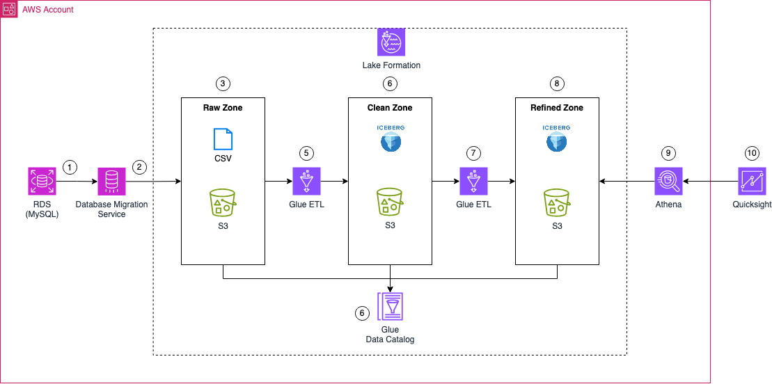
To achieve this, we’ll first create a Glue ETL job that processes data from the clean zone, consolidating it into a unified view before storing the results in an Apache Iceberg table within the refined zone. This refined zone acts as the foundation for our Business Intelligence workloads, making it easier to access and analyze data efficiently.
From there, the consolidated data will be accessed by Amazon QuickSight via an Athena data connection. QuickSight will allow us to visualize the refined data, making analysis more intuitive and helping us extract meaningful insights.
Note
The foundational setup for this project was completed in Parts 1 and 2. By now, you should have a working AWS DMS ingestion pipeline, along with a Glue ETL job that has populated the clean zone and updated the Glue Data Catalog. If you haven’t completed these steps yet, please go back to Parts 1 and 2 before proceeding.
Bootstrap Environment
Note
The Terraform code in this example is not divided into multiple parts. Instead, deploying the Terraform configuration will provision all components required for Part 1, Part 2, and Part 3 of this blog series.
The environment should already be set up as part of Part 1 of this series. If not, please return to Part 1 and complete the prerequisite steps before proceeding. This includes setting up AWS DMS for data ingestion and ensuring the initial pipeline is operational. Once those steps are completed, you’ll be ready to continue with Part 3.
To avoid unnecessary costs, please ensure that you destroy the infrastructure once you have completed the deployment and testing.
Recap
As mentioned earlier, the infrastructure was already set up in Part 1 of this series. Therefore, no additional infrastructure needs to be created in this section.
To recap, we initially created three tables— sales, book, and customer —in our database. After inserting sample data, we performed a full load using AWS DMS. We then made the following changes:
- Inserted a new record into the book table and updated an existing one.
- Modified the schema by adding a publisher column to the book table.
- Inserted an additional record reflecting the schema change.
At this point, your data lake should contain the following files:
- bookstoredb/sales/LOAD00000001.csv – Full load file for the sales table.
- bookstoredb/book/LOAD00000001.csv – Full load file for the book table.
- bookstoredb/customer/LOAD00000001.csv – Full load file for the customer table.
- bookstoredb/book/TIMESTAMP_INSERT_UPDATE.csv – File generated from insert and update operations in the book table.
- bookstoredb/sales/TIMESTAMP_ALTER_TABLE_INSERT.csv – File generated after altering the book table and adding a new record.
This means your data lake should contain a total of five files.
In Part 2, we explored the Glue Jobs that were automatically triggered through EventBridge rules and AWS Step Functions. These jobs processed the raw data and transformed it into Apache Iceberg tables within the clean zone. They also updated the AWS Glue Data Catalog, making metadata management and querying seamless.
At this stage, your AWS Glue Data Catalog should contain the following tables:
- bookstoredb_book – Table created by the Glue Crawler, pointing to the raw zone book data.
- iceberg_bookstoredb_book – Iceberg table for book, created by the glue-init ETL job and updated by glue-incremental.
- bookstoredb_customer – Table created by the Glue Crawler, pointing to the raw zone customer data.
- iceberg_bookstoredb_customer – Iceberg table for customer, created by glue-init and updated by glue-incremental.
- bookstoredb_sales – Table created by the Glue Crawler, pointing to the raw zone sales data.
- iceberg_bookstoredb_sales – Iceberg table for sales, created by glue-init and updated by glue-incremental.
In total, your Glue Data Catalog should now contain six tables.
To ensure everything is working as expected, you can repeat the verification steps from the end of Part 2 to validate the data in your Iceberg tables. This will confirm that all transformations and schema updates were correctly applied.
Consolidate Data
After you have verified that the Iceberg tables are present and correct, we will continue with the analysis of the AWS Glue consolidate job. While the job has already been created as part of the infrastrucutre roll out in part 1 of this series, the job has not been triggered yet. Instead of being triggered automatically once new data arrives in the clean zone Iceberg tables, this job is triggerd on a schedule by EventBridge at midnight.
Navigate to the AWS Glue Console and select the consolidate Glue ETL job. Before starting the Glue job, lets dive a bit deeper into the actual code.
To better understand the workflow of the glue-consolidate job, lets take a look at the code.
import sys
import boto3
from awsglue.utils import getResolvedOptions
from pyspark.sql import SparkSession
from pyspark.sql.functions import col
from awsglue.context import GlueContext
from awsglue.job import Job
from pyspark.sql.functions import col


# Parse input arguments from AWS Glue job
args = getResolvedOptions(sys.argv, [
    'JOB_NAME',
    'sales_table_name',
    'customer_table_name',
    'book_table_name',
    'glue_database_name',
    'refined_zone_bucket_name',
    'catalog_name',
    'iceberge_consolidated_table_name'
])

# Assign arguments to variables
salesTableName = args['sales_table_name']
customerTableName = args['customer_table_name']
bookTableName = args['book_table_name']
glueDatabaseName = args['glue_database_name']
refinedZoneBucketName = args['refined_zone_bucket_name']
catalog_name = args['catalog_name']

icebergTableName = args['iceberge_consolidated_table_name']
icebergS3Location = f"s3://{refinedZoneBucketName}/{icebergTableName}/"

# Initialize Spark Session with Iceberg configurations

spark = SparkSession.builder \
    .config(f"spark.sql.catalog.{catalog_name}", "org.apache.iceberg.spark.SparkCatalog") \
    .config(f"spark.sql.catalog.{catalog_name}.warehouse", icebergS3Location) \
    .config(f"spark.sql.catalog.{catalog_name}.catalog-impl", "org.apache.iceberg.aws.glue.GlueCatalog") \
    .config(f"spark.sql.catalog.{catalog_name}.io-impl", "org.apache.iceberg.aws.s3.S3FileIO") \
    .config(f"spark.sql.extensions", "org.apache.iceberg.spark.extensions.IcebergSparkSessionExtensions") \
    .getOrCreate()

# Initialize Spark & Glue Context
sc = spark.sparkContext
glueContext = GlueContext(sc)
job = Job(glueContext)
job.init(args['JOB_NAME'], args)


# Load Sales, Customer, and Book tables as DataFrames
sales_df = spark.read.format("iceberg") \
    .load(f"{catalog_name}.{glueDatabaseName}.{salesTableName}")

customer_df = spark.read.format("iceberg") \
    .load(f"{catalog_name}.{glueDatabaseName}.{customerTableName}")

book_df = spark.read.format("iceberg") \
    .load(f"{catalog_name}.{glueDatabaseName}.{bookTableName}")

# Rename columns in sales_df and customer_df before performing the join
sales_df_renamed = sales_df.withColumnRenamed("last_update_time", "sale_last_update_time")

customer_df_renamed = customer_df.withColumnRenamed("customer_id", "customer_customer_id") \
                                 .withColumnRenamed("last_update_time", "customer_last_update_time")

book_df_renamed = book_df.withColumnRenamed("book_id", "book_book_id") \
                                 .withColumnRenamed("last_update_time", "book_last_update_time")

# Perform the join with the renamed columns
sales_customer_join_df = sales_df_renamed.join(
    customer_df_renamed,
    sales_df_renamed["customer_id"] == customer_df_renamed["customer_customer_id"],
    "left"
)


# Perform Inner Join between Sales and Book on the common key
sales_complete_join_df = sales_customer_join_df.join(
    book_df_renamed,
    sales_df_renamed["book_id"] == book_df_renamed["book_book_id"],
    "left"
)

# Drop unneeded join columns
sales_complete_join_df = sales_complete_join_df.drop("book_book_id").drop("customer_customer_id")

# Register the DataFrame as a TempView
sales_complete_join_df.createOrReplaceTempView("OutputDataFrameTable")

# Step 6: Write the filtered data to an Iceberg table
create_table_query = f"""
    CREATE OR REPLACE TABLE {catalog_name}.`{glueDatabaseName}`.{icebergTableName}
    USING iceberg
    TBLPROPERTIES ("format-version"="2")
    AS SELECT * FROM OutputDataFrameTable;
    """

# Run the Spark SQL query
spark.sql(create_table_query)

#Update Table property to accept Schema Changes
spark.sql(f"""ALTER TABLE {catalog_name}.`{glueDatabaseName}`.{icebergTableName} SET TBLPROPERTIES (
                'write.spark.accept-any-schema'='true'
            )""")

job.commit()
Initialize Spark and Glue Context
- The job sets up a Spark session with Iceberg configurations, enabling AWS Glue to interact with Iceberg tables.
- The Glue job is initialized to manage execution.
spark = SparkSession.builder \
    .config(f"spark.sql.catalog.{catalog_name}", "org.apache.iceberg.spark.SparkCatalog") \
    .config(f"spark.sql.catalog.{catalog_name}.warehouse", icebergS3Location) \
    .config(f"spark.sql.catalog.{catalog_name}.catalog-impl", "org.apache.iceberg.aws.glue.GlueCatalog") \
    .config(f"spark.sql.catalog.{catalog_name}.io-impl", "org.apache.iceberg.aws.s3.S3FileIO") \
    .config(f"spark.sql.extensions", "org.apache.iceberg.spark.extensions.IcebergSparkSessionExtensions") \
    .getOrCreate()

sc = spark.sparkContext
glueContext = GlueContext(sc)
job = Job(glueContext)
job.init(args['JOB_NAME'], args)
Load Data from Iceberg Tables
- The script reads sales, customer, and book data into Spark DataFrames.
sales_df = spark.read.format("iceberg").load(f"{catalog_name}.{glueDatabaseName}.{salesTableName}")
customer_df = spark.read.format("iceberg").load(f"{catalog_name}.{glueDatabaseName}.{customerTableName}")
book_df = spark.read.format("iceberg").load(f"{catalog_name}.{glueDatabaseName}.{bookTableName}")
Rename Columns to Avoid Naming Conflicts
- To prevent duplicate column names after joins, certain fields are renamed.
sales_df_renamed = sales_df.withColumnRenamed("last_update_time", "sale_last_update_time")

customer_df_renamed = customer_df.withColumnRenamed("customer_id", "customer_customer_id") \
                                 .withColumnRenamed("last_update_time", "customer_last_update_time")

book_df_renamed = book_df.withColumnRenamed("book_id", "book_book_id") \
                         .withColumnRenamed("last_update_time", "book_last_update_time")
Perform Joins
- Join Sales and Customer Data (Left Join)
- Join Sales-Customer Data with Book Data (Left Join)
- After the joins, unnecessary columns are dropped to keep only relevant data.
sales_customer_join_df = sales_df_renamed.join(
    customer_df_renamed,
    sales_df_renamed["customer_id"] == customer_df_renamed["customer_customer_id"],
    "left"
)

sales_complete_join_df = sales_customer_join_df.join(
    book_df_renamed,
    sales_df_renamed["book_id"] == book_df_renamed["book_book_id"],
    "left"
)

sales_complete_join_df = sales_complete_join_df.drop("book_book_id").drop("customer_customer_id")
Write Processed Data to an Iceberg Table
- The final DataFrame is registered as a temporary view for SQL operations.
- The table is created or replaced with the transformed data.
- To support schema evolution, the table properties are updated.
sales_complete_join_df.createOrReplaceTempView("OutputDataFrameTable")

create_table_query = f"""
    CREATE OR REPLACE TABLE {catalog_name}.`{glueDatabaseName}`.{icebergTableName}
    USING iceberg
    TBLPROPERTIES ("format-version"="2")
    AS SELECT * FROM OutputDataFrameTable;
    """
spark.sql(create_table_query)

spark.sql(f"""ALTER TABLE {catalog_name}.`{glueDatabaseName}`.{icebergTableName} SET TBLPROPERTIES (
                'write.spark.accept-any-schema'='true'
            )""")
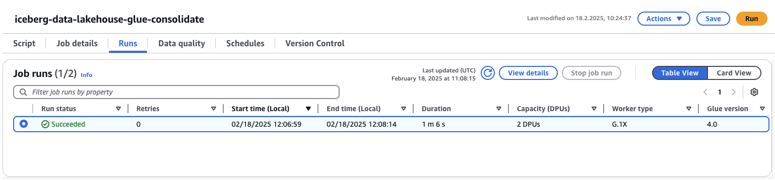
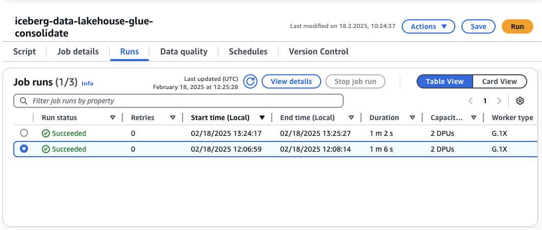
Select the job and click on Run in the top right corner. The job should start and succeed after about 1 or 2 minutes.
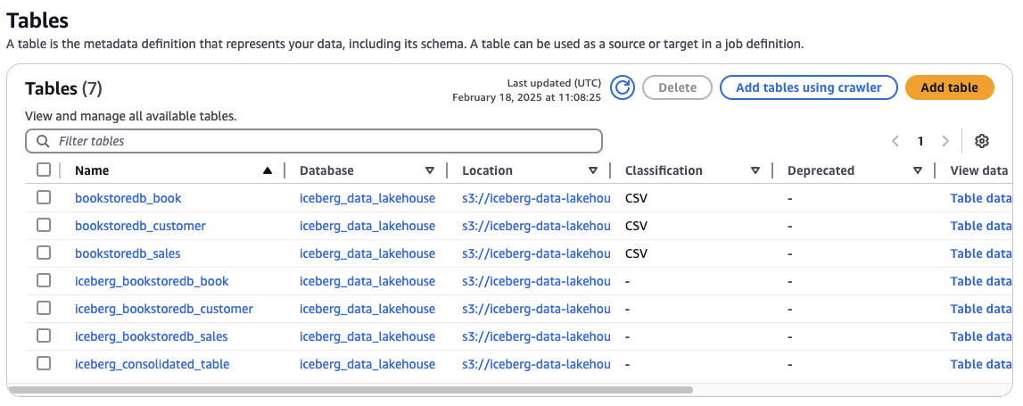
Navigate to the AWS Glue Data Catalog and you should see that a new table called siceberg_consolidated_tables has been created. This table houses the joined data from the sales, book, and customer Iceberg tables from the clean zone.
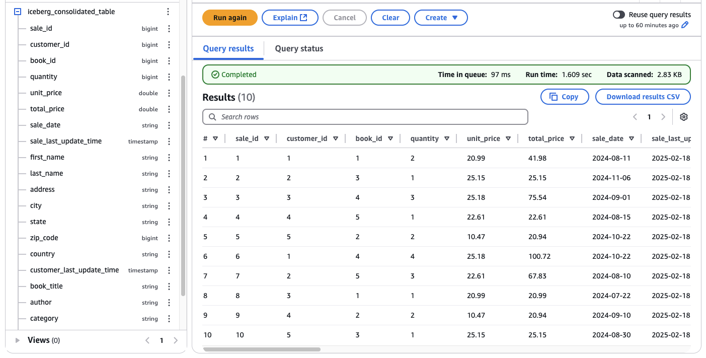
Before creating the Quicksight dashboard, we will verify the data by using Athena. Navigate to the Athena console, select the table iceberg_consolidated_table, and click on Preview Table. Athena should list the first 10 entries of the table. As you can see, this table is a flat table and a combination of the three tables sales, book, and customer. By flattening and joining the table at this stage, we prevent extra work in Quicksight and ensure that changes are performed within the data lake and close to the source.
Setup QuickSight Dashboard (Optional)
Note
The next two sections are optional. If you do not wish to enable QuickSight, you can skip them. In this case, congratulations! You have successfully set up a fully functional data lake that supports ingestion, storage, and processing while also providing data for downstream workloads.
We will now continue by setting up a QuickSight Dashboard. Start by navigating to the AWS QuickSight console. If you haven’t created a QuickSight account yet, go ahead and do so. Don’t worry—you can delete the account once you’ve completed this demonstration. After logging in, we need to grant your QuickSight user access to the data lake before moving forward. Open the quicksight.tf file and remove the comments at the beginning and end of the file. Inside, you’ll find a locals block where you should replace the placeholder xxxxxxxxxxxxxxxxxx with your own quicksight_user_name to provide access to the refined zone data in the data lake.
locals {
  quicksight_user_name = "xxxxxxxxxxxxxxxxxx"
}
Once you’ve updated the file, save it and run terraform apply. This command will deploy the necessary infrastructure, updating AWS LakeFormation permissions and granting your QuickSight user access to the required data.
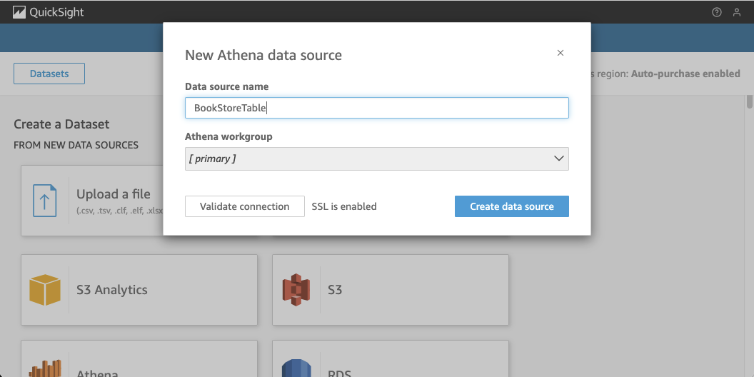
Now that your QuickSight user has the correct permissions, we can create a new dataset in QuickSight using Athena as the data source. Be sure to select the same region as your data lake when proceeding. In the QuickSight console, navigate to Datasets, and click on New dataset in the top right corner. Choose Athena as the data source and assign a name to your dataset, then click Create data source.
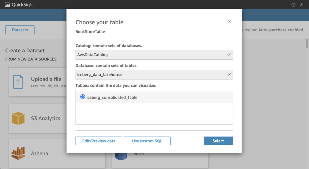
In the next window, select the appropriate database, iceberg_data_lakehouse, and the iceberg_consolidated_table as your data source. Once you’ve configured this, click Select.
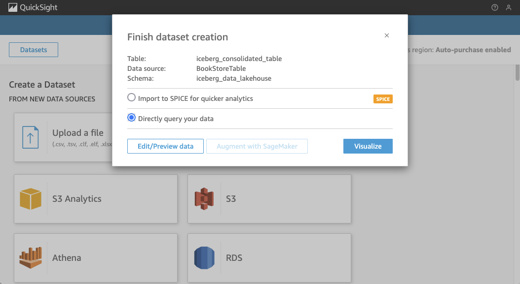
On the final screen, choose Directly query our data, as we won’t be using SPICE in this example. Click Visualize to begin building your dashboard.
Note
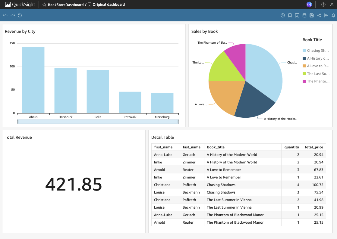
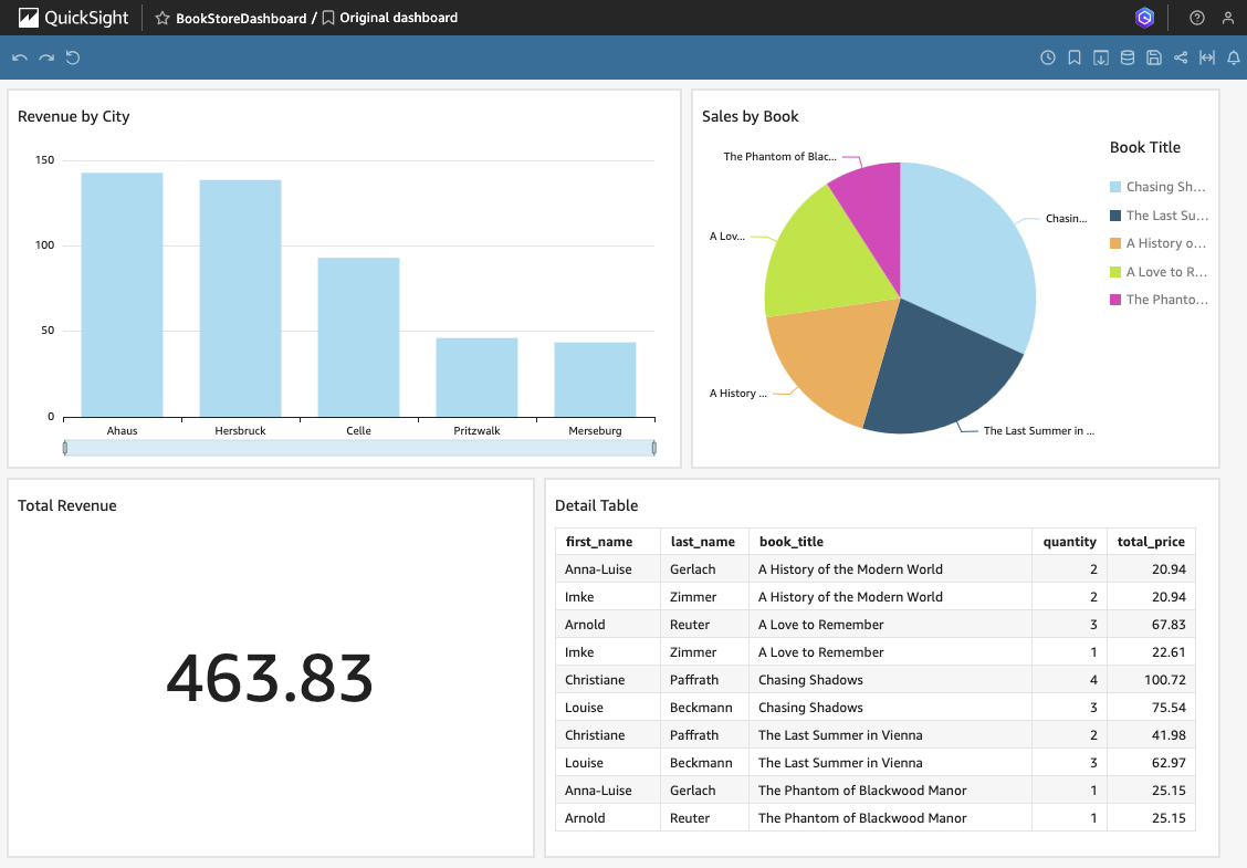
This guide doesn’t go into detail on how to use QuickSight. Feel free to either build your own dashboard or use the sample provided below.
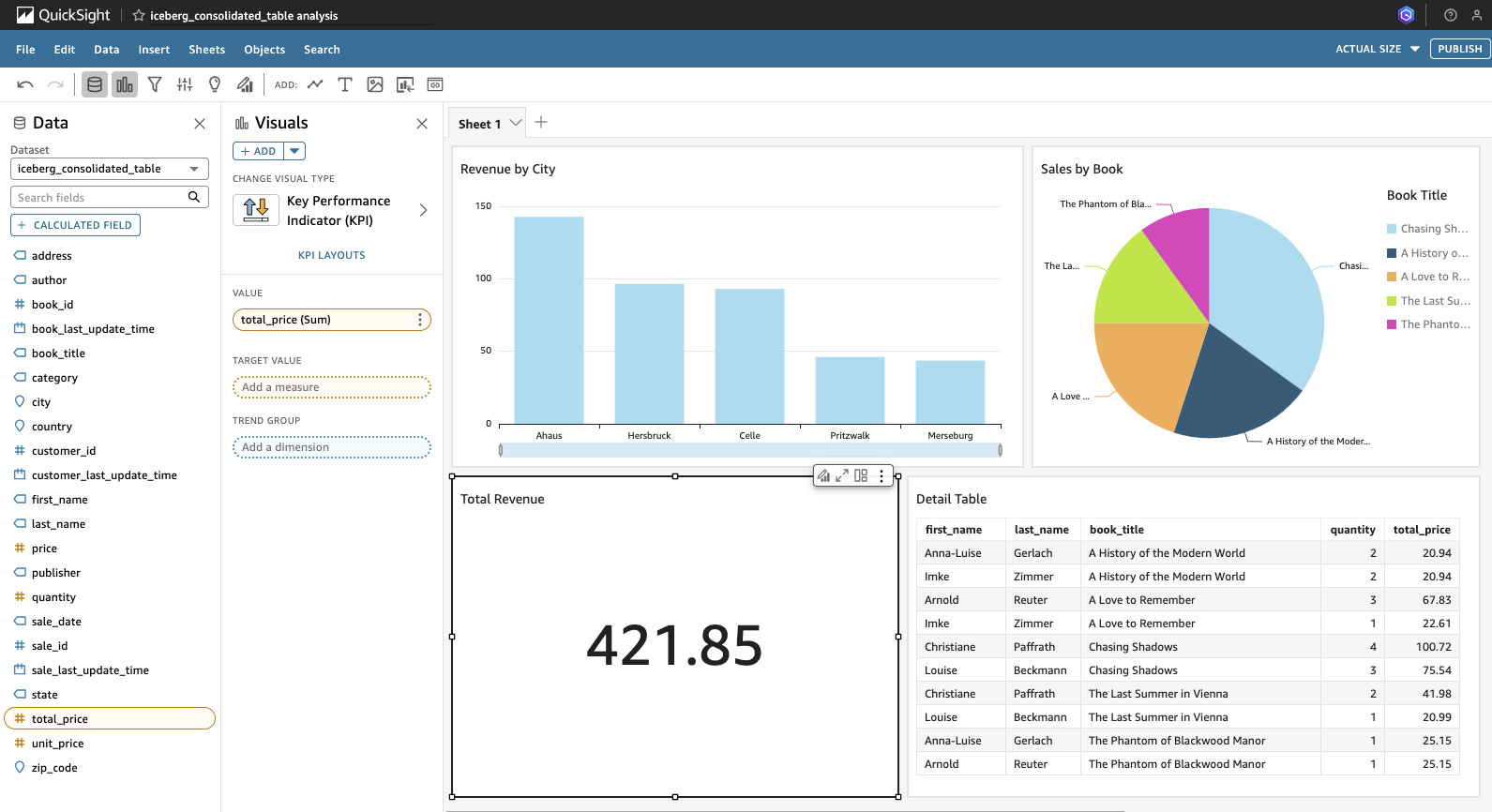
After building your dashboard, click Publish in the top right corner to finalize your work. Assign a name to the dashboard and click Publish dashboard to make it available.
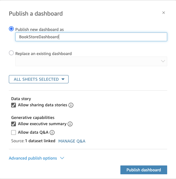
Your dashboard should now appear under the Dashboards section in QuickSight, where you can begin utilizing it to gain insights into your bookstore sales data.
Update QuickSight Dashboard (Optional)
To drive home the process of how data moves from the MySQL database into the data lake via AWS DMS and finally ends up in the QuickSight dashboard using Glue ETL transformations, we will go back to the beginning and add some data to the source database. This data should later be viewable in the dashboard once the workflow has been successfully finsihed.
Open the database connection window. Return the part 1 of this series if you need a refreseher. Execute the following SQL statement to insert a new entry into the sales table:
INSERT INTO sales (customer_id, book_id, quantity, unit_price, total_price, sale_date)
VALUES
    (3, 1, 2, 20.99, 41.98, '2025-02-18') -- Louise Beckmann buys 2 additional copies of 'The Last Summer in Vienna'
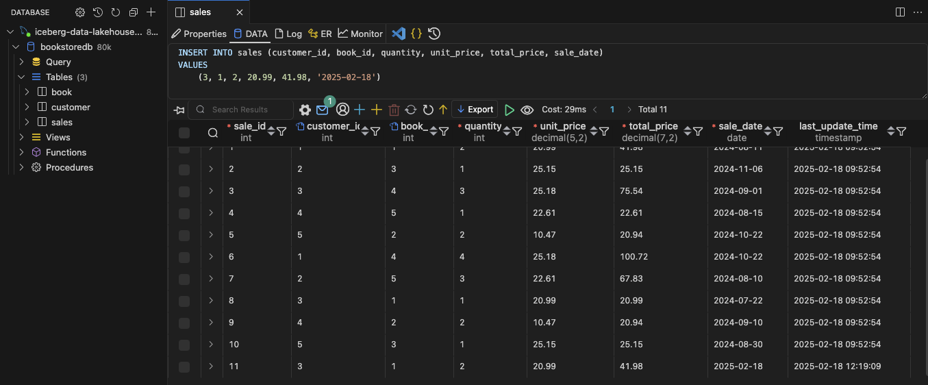
Once the data has been added, wait a moment for DMS to pick up the changes and for the Glue job glue-incremental to add the new entry to the Iceberg sales table. Navigate to the AWS Glue console and continue once the Glue job glue-incremental had run and finished succesfully. Afterward, we will rerun the Glue job consolidate. Select the Glue job consolidate and click on Run to run the job. Wait for the job to finish succesfully. The consolidated table our Quicksight dashboard is based on should now be up to date.
Return to your Quicksight dashboard and refresh the page. As we selected Directly query our data when creating the dataset, the data will now be loaded fresh using Athena in the backgroud. As you can see, the sales values have increased. You will also notice that Louse Beckmann has now bought three copies of The Last Summer in Vienna instead of one. this is a confirmation, that our complete pipeline is working as expected.
Clean up
To clean up the environment, simply run terraform destroy in the cloned repository. This will remove all the resources that were created during the setup process.
Warning
Since QuickSight was not set up using Terraform, please remember to close your QuickSight account after completing this example if you no longer wish to use the service.
Summary
Congratulations on completing the last part of this three-part series!
In this third blog post, we complete the series by integrating a Business Intelligence (BI) workload into our transactional Data Lake. Building on the previous steps, we consolidate data stored in Apache Iceberg tables and use it as the foundation for a QuickSight dashboard. This allows us to visualize the data and gain valuable insights, providing a powerful, high-performance solution for running analytics on our data lake. By integrating QuickSight, we enhance our Data Lake with BI capabilities, making it easier to derive actionable insights from the transactional data stored in Amazon S3.
I hope you enjoyed this example and learned something new. I look forward to your feedback and questions. For the complete example code, please visit my Github.
— Hendrik
Title Photo by Sophie Turner on Unsplash